Inventory

A R-package for Modeling emission inventories from geographic data.

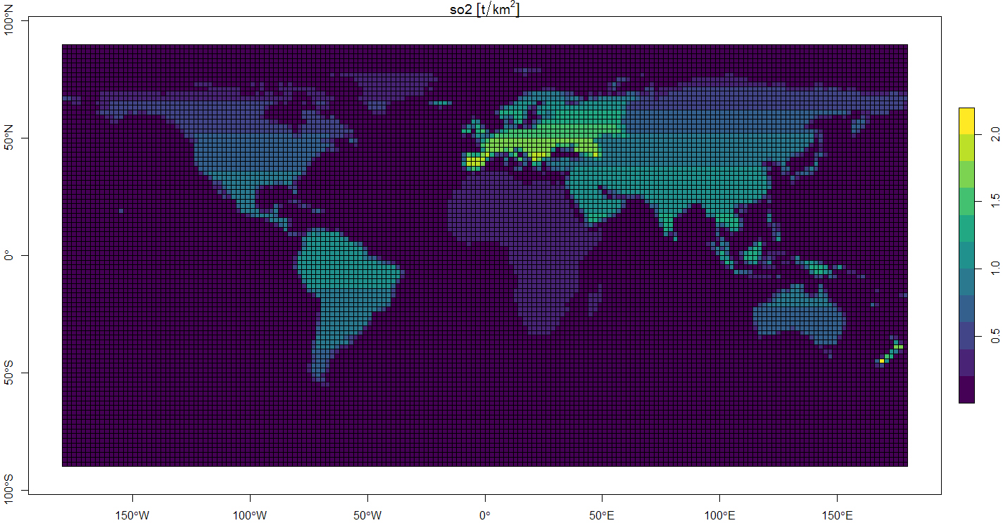
Figure 1 shows an example of global inventory, this emission was generated with the code bellow:

# load this package
library(inventory)
# open a shapefile and selecting the desired region
continents <- sf::st_read(paste0(system.file("extdata",package="inventory"),"/continent.shp"))
continents <- continents[-8,]
# open and selecting the emission data to be used in inventory
so2 <- read.csv(paste0(system.file("extdata",package="inventory"),"/SO2.csv"))
names(so2) <- c("region","year","mass")
so2 <- so2[so2$year == 2010,]
so2$region <- as.character(so2$region)
# add some arbitrary data
so2 <- rbind(so2,c("Oceania",   2010,0.0002 * as.numeric(so2$mass[1])))
so2 <- rbind(so2,c("Australia", 2010,0.0200 * as.numeric(so2$mass[1])))
so2$mass[3] <- as.numeric(so2$mass[3]) / 4

# organize data for inventory
so2_2010 <- geoemiss(geom     = continents,
                     values   = so2$mass,
                     names    = so2$region,
                     variable = "so2")

# make a global inventory of so2 with 2 degrees of resolution 
inventory_res_2 <- griding(so2_2010,"so2", res = 2)

# visualize the output
# install.packages("cptcity")
library(cptcity)
plot(inventory_res_2["so2"], axes = T, pal = cpt(pal = 920,colorRampPalette = T))

# to save the output in NetCDF-4 format (ask for the file name/location)
saveInventory(inventory_res_2,variable = "so2",dates = '2010-01-01',mw = 64.066)

The creation of the emissions follows 3 steps process: pre-processing the input data by geoemiss(), generate the grid and distribute the emission by the sum of interssections of grid and regions by griding(), and save the output and metadata with saveInventory(). Figure 2 shows a diagram of the prosses, the circles represents input and output files, the boxes represents functions, and the gray color are used in optional steps.

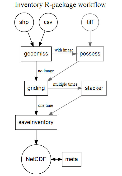
Figure 2 includes 3 additional prosses that can be apply to the inventory:

• The use of an additional layer with a georeferenced immage to improve the distribution inside big flat areas using the possess() function before the griding() function;
• A way to stack many times to record in one output file with the function stacker() before saveInventory();
• A way to read and write metada to the final NetCDF file with the function meta().

Figure 2 shows a example of local inventory for two Brazilian states (São Paulo and Rio de Janeiro) using a additional image layer of Images from the Defense Meteorological Satellite Program (DMSP).

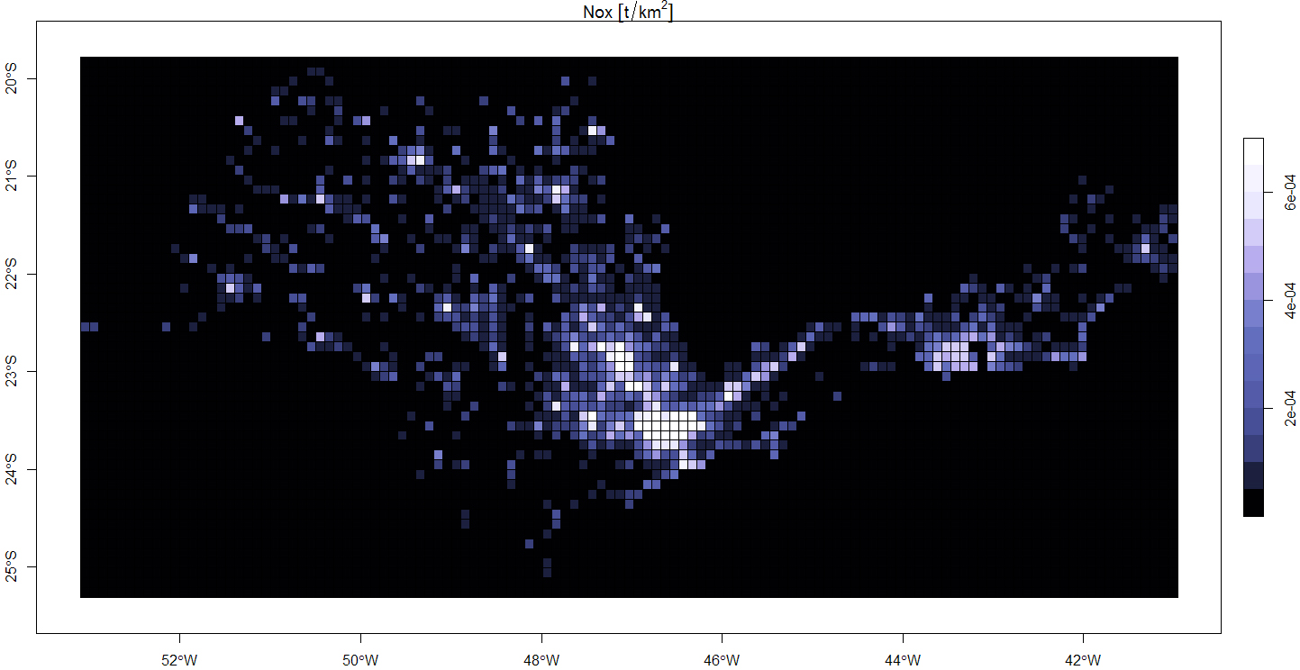
generated by the code bellow:

library(inventory)
# read a shapefile with shapes of the 2 states
states <- sf::st_read(paste(system.file("extdata", package = "inventory"),"/states.shp",sep=""))
# processes the input data
Nox    <- geoemiss(geom = states,variable = "Nox",names = c("sp","rj"),values = c(1000,25))
# file name for this example
image  <- paste(system.file("extdata", package = "inventory"),"/tiny.tif",sep="")
# read and process the image
ras    <- possess(Nox,image,plots = F)
# calculate the local inventory with 0.1 of resolution 
local  <- griding(ras,variable = "Nox", res = 0.1, type = "local", plot = F)
# visualize
# install.packages("cptcity")
library(cptcity)
plot(local["Nox"], axes = T,pal = cpt(pal = 6101,colorRampPalette = T))

Installation

System dependencies

inventory import functions from ncdf4 for reading model information, raster and sf to process grinded/geographic information and units. These packages need some additional libraries:

To Ubuntu

The following steps are required for installation on Ubuntu:

  sudo add-apt-repository ppa:ubuntugis/ubuntugis-unstable --yes
  sudo apt-get --yes --force-yes update -qq
  # netcdf dependencies:
  sudo apt-get install --yes libnetcdf-dev netcdf-bin
  # units/udunits2 dependency:
  sudo apt-get install --yes libudunits2-dev
  # sf dependencies (without libudunits2-dev):
  sudo apt-get install --yes libgdal-dev libgeos-dev libproj-dev

To Fedora

The following steps are required for installation on Fedora:

  sudo dnf update
  # netcdf dependencies:
  sudo yum install netcdf-devel
  # units/udunits2 dependency:
  sudo yum install udunits2-devel
  # sf dependencies (without libudunits2-dev):
  sudo yum install gdal-devel proj-devel proj-epsg proj-nad geos-devel

To Windows

No additional steps for windows installation.

Detailed instructions can be found at netcdf, libudunits2-dev and sf developers page.

Package installation

# install.packages("devtools")
devtools::install_github("schuch666/inventory")

Licence

Licensed under a Creative Commons Attribution 4.0 International License (CC BY).