Distribute emissions into grids

calculate the inventory from a geoemiss ouput, there is 3 grid types: - global: cover all latitudes and longitudes - local: cover the latitudes and longitudes of the input data - custom: with custom limits

res argument controls the resolution of the final grid, grids whith higher resolution take more time to calculate

griding(geoemiss, variable = NA, area_unit = "km^2", res = 5,
  type = "global", lat = c(-90, 90), lon = c(-180, 180), tol = res
  * 1e-05, verbose = T, plot = F, ...)

Arguments

geoemiss	a sf from geoemiss
variable	name(s) of the pollutant(s)
area_unit	area unit, default is "km^2"
res	inventory resolution in degrees
type	global, local or custom inventary type
lat	latitude for custom inventory
lon	lontitude for custom inventory
tol	param passing to dist of sf::st_buffer
verbose	display additional information
plot	true for plot separate regions and the final inventory
...	additional plot parameters

Value

a sf with the grid geometry and the emission by cell

Note

inventories with multiple dates need to be combined with stacker function

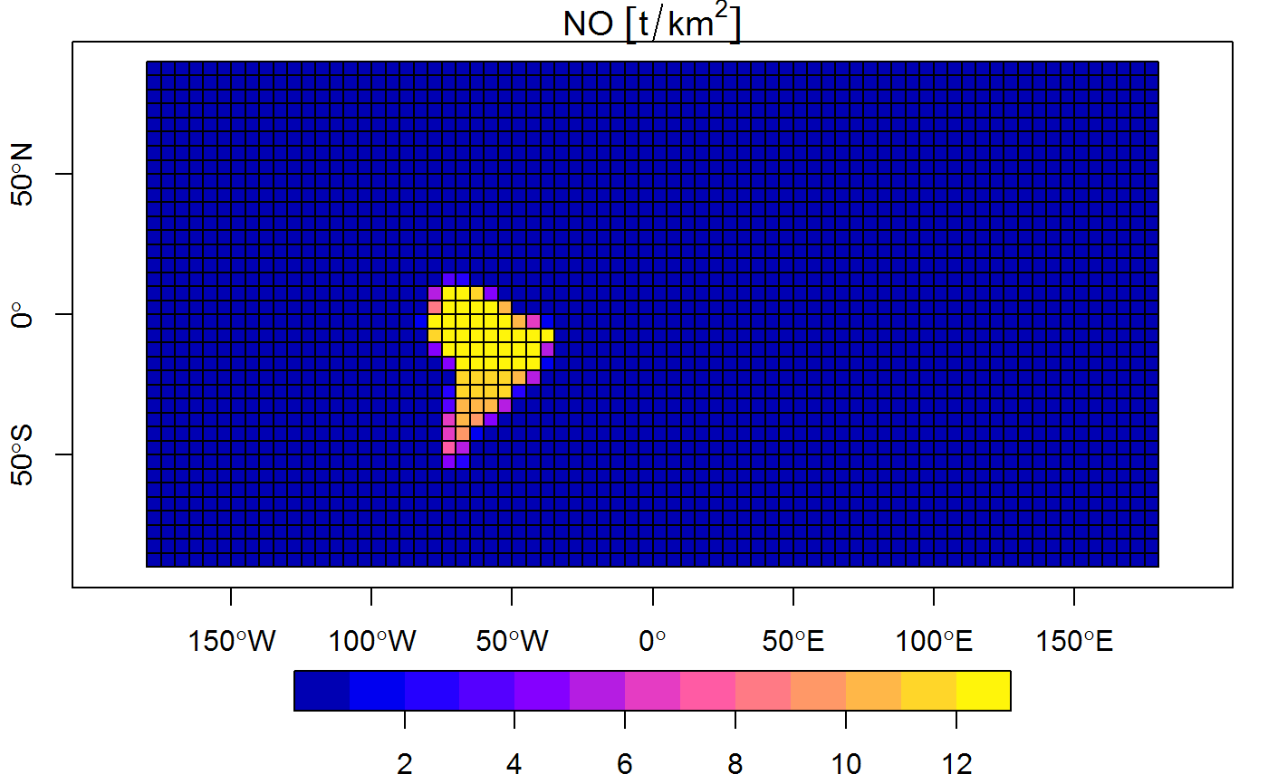
Examples

so2_no_2010 <- readRDS(paste0(system.file("extdata",package="inventory"),"/so2_no.Rds"))
inventory_so2_2010 <- griding(so2_no_2010[5,], variable = c("so2","NO"), plot = TRUE)
#> processing South America area ...
#> Linking to GEOS 3.6.1, GDAL 2.2.3, proj.4 4.9.3
#> dist is assumed to be in decimal degrees (arc_degrees).
#> although coordinates are longitude/latitude, st_intersection assumes that they are planar